Activation functions in Neural Networks

Sébastien De Greef

Activation functions

When choosing an activation function, consider the following:

  • Non-saturation: Avoid activations that saturate (e.g., sigmoid, tanh) to prevent vanishing gradients.

  • Computational efficiency: Choose activations that are computationally efficient (e.g., ReLU, Swish) for large models or real-time applications.

  • Smoothness: Smooth activations (e.g., GELU, Mish) can help with optimization and convergence.

  • Domain knowledge: Select activations based on the problem domain and desired output (e.g., softmax for multi-class classification).

  • Experimentation: Try different activations and evaluate their performance on your specific task.

Sigmoid

  • Strengths: Maps any real-valued number to a value between 0 and 1, making it suitable for binary classification problems.

  • Weaknesses: Saturates (i.e., output values approach 0 or 1) for large inputs, leading to vanishing gradients during backpropagation.

  • Usage: Binary classification, logistic regression.

\[ \sigma(x) = \frac{1}{1 + e^{-x}} \]

def sigmoid(x):
    return 1 / (1 + np.exp(-x))
Figure 1: Sigmoid Functions

Hyperbolic Tangent (Tanh)

Strengths: Similar to sigmoid, but maps to (-1, 1), which can be beneficial for some models.

Weaknesses: Also saturates, leading to vanishing gradients.

Usage: Similar to sigmoid, but with a larger output range.

\[ \tanh(x) = \frac{e^{x} - e^{-x}}{e^{x} + e^{-x}} \]

def tanh(x):
    return np.tanh(x)
Figure 2: Hyperbolic Tangent

Rectified Linear Unit (ReLU)

Strengths: Computationally efficient, non-saturating, and easy to compute.

Weaknesses: Not differentiable at x=0, which can cause issues during optimization.

Usage: Default activation function in many deep learning frameworks, suitable for most neural networks.

\[ \text{ReLU}(x) = \max(0, x) \]

def relu(x):
    return np.maximum(0, x)
Figure 3: ReLU and Variants

Leaky ReLU

Strengths: Similar to ReLU, but allows a small fraction of the input to pass through, helping with dying neurons.

Weaknesses: Still non-differentiable at x=0.

Usage: Alternative to ReLU, especially when dealing with dying neurons.

\[ \text{Leaky ReLU}(x) = \begin{cases} x & \text{if } x > 0 \\ \alpha x & \text{if } x \leq 0 \end{cases} \]

def leaky_relu(x, alpha=0.01):
    # where α is a small constant (e.g., 0.01)
    return np.where(x > 0, x, x * alpha)
Figure 4: Leaky Relu

Swish

Strengths: Self-gated, adaptive, and non-saturating.

Weaknesses: Computationally expensive, requires additional learnable parameters.

Usage: Can be used in place of ReLU or other activations, but may not always outperform them.

\[ \text{Swish}(x) = x \cdot \sigma(x) \]

def swish(x):
    return x * sigmoid(x)

See also: sigmoid

Figure 5: Swish

Mish

Strengths: Non-saturating, smooth, and computationally efficient.

Weaknesses: Not as well-studied as ReLU or other activations.

Usage: Alternative to ReLU, especially in computer vision tasks.

\[ \text{Mish}(x) = x \cdot \tanh(\text{Softplus}(x)) \]

def mish(x):
    return x * np.tanh(softplus(x))
Figure 6: Mish

See also: softplus tanh

Softmax

Strengths: Normalizes output to ensure probabilities sum to 1, making it suitable for multi-class classification.

Weaknesses: Only suitable for output layers with multiple classes.

Usage: Output layer activation for multi-class classification problems.

\[ \text{Softmax}(x_i) = \frac{e^{x_i}}{\sum_{k=1}^{K} e^{x_k}} \]

def softmax(x):
    e_x = np.exp(x - np.max(x))
    return e_x / e_x.sum()
Figure 7: SoftMax

Softsign

Strengths: Similar to sigmoid, but with a more gradual slope.

Weaknesses: Not commonly used, may not provide significant benefits over sigmoid or tanh.

Usage: Alternative to sigmoid or tanh in certain situations.

\[ \text{Softsign}(x) = \frac{x}{1 + |x|} \]

def softsign(x):
    return x / (1 + np.abs(x))
Figure 8: SoftSign

SoftPlus

Strengths: Smooth, continuous, and non-saturating.

Weaknesses: Not commonly used, may not outperform other activations.

Usage: Experimental or niche applications.

\[ \text{Softplus}(x) = \log(1 + e^x) \]

def softplus(x):
    return np.log1p(np.exp(x))
Figure 9: SoftPlus

ArcTan

Strengths: Non-saturating, smooth, and continuous.

Weaknesses: Not commonly used, may not outperform other activations.

Usage: Experimental or niche applications.

\[ arctan(x) = arctan(x) \]

def arctan(x):
    return np.arctan(x)
Figure 10: Arc Tangent

Gaussian Error Linear Unit (GELU)

Strengths: Non-saturating, smooth, and computationally efficient.

Weaknesses: Not as well-studied as ReLU or other activations.

Usage: Alternative to ReLU, especially in Bayesian neural networks.

\[ \text{GELU}(x) = x \cdot \Phi(x) \]

def gelu(x):
    return 0.5 * x 
        * (1 + np.tanh(np.sqrt(2 / np.pi) 
        * (x + 0.044715 * np.power(x, 3))))
Figure 11: GeLU

See also: tanh

Silu (SiLU)

\[ silu(x) = x * sigmoid(x) \]

Strengths: Non-saturating, smooth, and computationally efficient.

Weaknesses: Not as well-studied as ReLU or other activations.

Usage: Alternative to ReLU, especially in computer vision tasks.

GELU Approximation (GELU Approx.)

\[ f(x) ≈ 0.5 * x * (1 + tanh(√(2/π) * (x + 0.044715 * x^3))) \]

Strengths: Fast, non-saturating, and smooth.

Weaknesses: Approximation, not exactly equal to GELU.

Usage: Alternative to GELU, especially when computational efficiency is crucial.

SELU (Scaled Exponential Linear Unit)

\[ f(x) = \lambda \begin{cases} x & x > 0 \\ \alpha e^x - \alpha & x \leq 0 \end{cases} \]

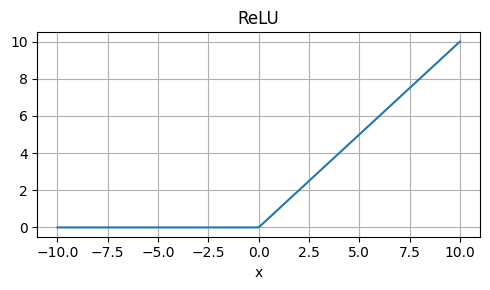
Strengths: Self-normalizing, non-saturating, and computationally efficient.

Weaknesses: Requires careful initialization and α tuning.

Usage: Alternative to ReLU, especially in deep neural networks.

I will incorporate a timeline diagram using Mermaid to visually represent the key milestones in the history of AI. Here’s the updated plan with the inclusion of the timeline, and I’ll proceed to create the detailed content for the slideshow afterward.

Detailed Slideshow Plan

  1. Introduction to AI
    • Define AI and its importance in modern technology.
  2. Early Concepts and Theoretical Foundations
    • Discuss the philosophical roots and ideas like the Turing Test.
  3. The Birth of AI: The Dartmouth Conference
    • Details on the 1956 Dartmouth workshop and its contributions.
  4. Early Successes and Challenges
    • Initial achievements and the subsequent AI winters.
  5. Rise of Machine Learning
    • Shift from symbolic AI to machine learning paradigms.
  6. AI Goes Mainstream: 2000s to Present
    • Highlight key advancements and the proliferation of AI in various sectors.
  7. Ethical Considerations and Future Outlook
    • Explore the ethical dilemmas and future possibilities.
  8. Conclusion
    • Summarize the evolution and impact of AI.

Timeline Diagrams

  • Key moments from the early theoretical concepts to the latest developments in AI will be represented in a Mermaid timeline for visual impact.

Now, I’ll gather the necessary information to fill in these sections and create the Mermaid timeline. Once the content is prepared, I’ll compile it into a format suitable for a slideshow. Let’s start with the first section, “Introduction to AI,” and proceed from there. Here’s the detailed content for the introduction:

Slide 1: Introduction to Artificial Intelligence

  • Title: Introduction to Artificial Intelligence
  • Content:
    • Definition: Artificial Intelligence (AI) involves creating computer systems that can perform tasks that typically require human intelligence. These tasks include decision-making, object detection, speech recognition, and language translation.
    • Impact: AI transforms industries including healthcare, automotive, finance, and entertainment by automating processes and analyzing large amounts of data with speed and accuracy beyond human capability.

Following this, I’ll move on to the historical aspects and then integrate the timeline. Would you like to add any specific details or case studies to the introduction or other sections?