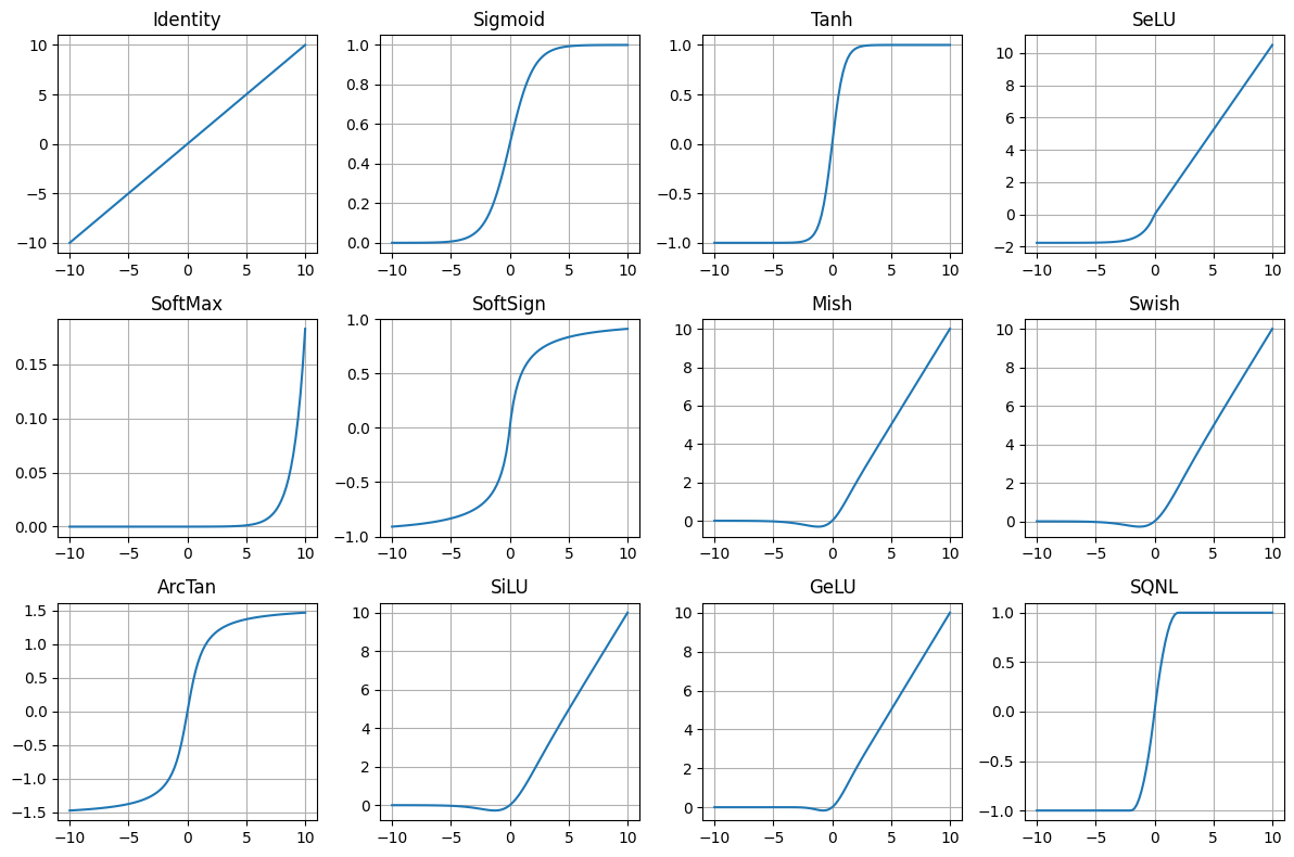
Activation functions
When choosing an activation function, consider the following:
Non-saturation: Avoid activations that saturate (e.g., sigmoid, tanh) to prevent vanishing gradients.
Computational efficiency: Choose activations that are computationally efficient (e.g., ReLU, Swish) for large models or real-time applications.
Smoothness: Smooth activations (e.g., GELU, Mish) can help with optimization and convergence.
Domain knowledge: Select activations based on the problem domain and desired output (e.g., softmax for multi-class classification).
Experimentation: Try different activations and evaluate their performance on your specific task.
Sigmoid
Strengths: Maps any real-valued number to a value between 0 and 1, making it suitable for binary classification problems.
Weaknesses: Saturates (i.e., output values approach 0 or 1) for large inputs, leading to vanishing gradients during backpropagation.
Usage: Binary classification, logistic regression.
\[ \sigma(x) = \frac{1}{1 + e^{-x}} \]
def sigmoid(x):
    return 1 / (1 + np.exp(-x))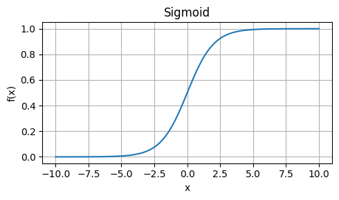
Hyperbolic Tangent (Tanh)
Strengths: Similar to sigmoid, but maps to (-1, 1), which can be beneficial for some models.
Weaknesses: Also saturates, leading to vanishing gradients.
Usage: Similar to sigmoid, but with a larger output range.
\[ \tanh(x) = \frac{e^{x} - e^{-x}}{e^{x} + e^{-x}} \]
def tanh(x):
    return np.tanh(x)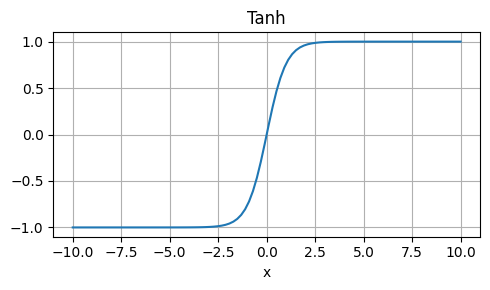
Rectified Linear Unit (ReLU)
Strengths: Computationally efficient, non-saturating, and easy to compute.
Weaknesses: Not differentiable at x=0, which can cause issues during optimization.
Usage: Default activation function in many deep learning frameworks, suitable for most neural networks.
\[ \text{ReLU}(x) = \max(0, x) \]
def relu(x):
    return np.maximum(0, x)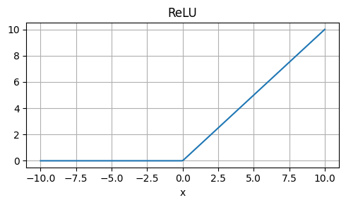
Leaky ReLU
Strengths: Similar to ReLU, but allows a small fraction of the input to pass through, helping with dying neurons.
Weaknesses: Still non-differentiable at x=0.
Usage: Alternative to ReLU, especially when dealing with dying neurons.
\[ \text{Leaky ReLU}(x) = \begin{cases} x & \text{if } x > 0 \\ \alpha x & \text{if } x \leq 0 \end{cases} \]
def leaky_relu(x, alpha=0.01):
    # where α is a small constant (e.g., 0.01)
    return np.where(x > 0, x, x * alpha)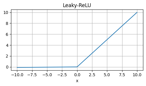
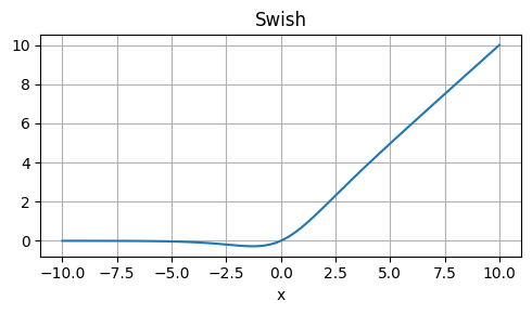
Swish
Formula:
where g(x) is a learned function (e.g., sigmoid or ReLU)
Strengths: Self-gated, adaptive, and non-saturating.
Weaknesses: Computationally expensive, requires additional learnable parameters.
Usage: Can be used in place of ReLU or other activations, but may not always outperform them.
Mish
Strengths: Non-saturating, smooth, and computationally efficient.
Weaknesses: Not as well-studied as ReLU or other activations.
Usage: Alternative to ReLU, especially in computer vision tasks.
\[ \text{Mish}(x) = x \cdot \tanh(\text{Softplus}(x)) \]
def mish(x):
    return x * np.tanh(softplus(x))
Softmax
Strengths: Normalizes output to ensure probabilities sum to 1, making it suitable for multi-class classification.
Weaknesses: Only suitable for output layers with multiple classes.
Usage: Output layer activation for multi-class classification problems.
\[ \text{Softmax}(x_i) = \frac{e^{x_i}}{\sum_{k=1}^{K} e^{x_k}} \]
def softmax(x):
    e_x = np.exp(x - np.max(x))
    return e_x / e_x.sum()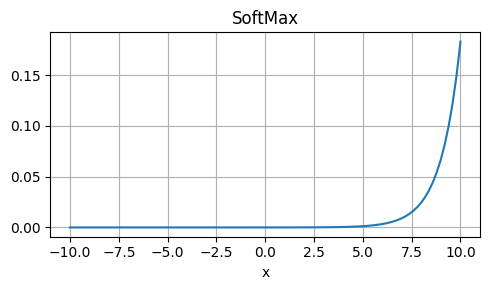
Softsign
Strengths: Similar to sigmoid, but with a more gradual slope.
Weaknesses: Not commonly used, may not provide significant benefits over sigmoid or tanh.
Usage: Alternative to sigmoid or tanh in certain situations.
\[ \text{Softsign}(x) = \frac{x}{1 + |x|} \]
def softsign(x):
    return x / (1 + np.abs(x))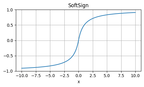
SoftPlus
Strengths: Smooth, continuous, and non-saturating.
Weaknesses: Not commonly used, may not outperform other activations.
Usage: Experimental or niche applications.
\[ \text{Softplus}(x) = \log(1 + e^x) \]
def softplus(x):
    return np.log1p(np.exp(x))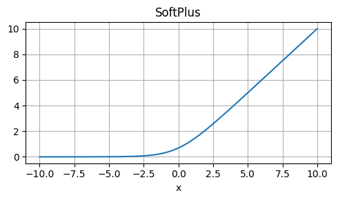
ArcTan
Strengths: Non-saturating, smooth, and continuous.
Weaknesses: Not commonly used, may not outperform other activations.
Usage: Experimental or niche applications.
\[ arctan(x) = arctan(x) \]
def arctan(x):
    return np.arctan(x)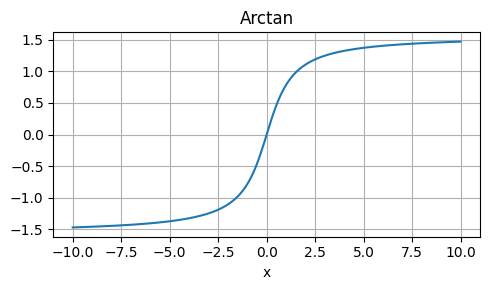
Gaussian Error Linear Unit (GELU)
Strengths: Non-saturating, smooth, and computationally efficient.
Weaknesses: Not as well-studied as ReLU or other activations.
Usage: Alternative to ReLU, especially in Bayesian neural networks.
\[ \text{GELU}(x) = x \cdot \Phi(x) \]
def gelu(x):
    return 0.5 * x
        * (1 + np.tanh(np.sqrt(2 / np.pi)
        * (x + 0.044715 * np.power(x, 3))))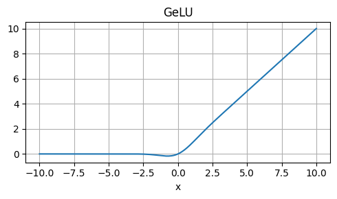
See also: tanh
Silu (SiLU)
Strengths: Non-saturating, smooth, and computationally efficient.
Weaknesses: Not as well-studied as ReLU or other activations.
Usage: Alternative to ReLU, especially in computer vision tasks.
\[ silu(x) = x * sigmoid(x) \]
def silu(x):
    return x / (1 + np.exp(-x))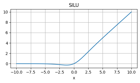
GELU Approximation (GELU Approx.)
\[ f(x) ≈ 0.5 * x * (1 + tanh(√(2/π) * (x + 0.044715 * x^3))) \]
Strengths: Fast, non-saturating, and smooth.
Weaknesses: Approximation, not exactly equal to GELU.
Usage: Alternative to GELU, especially when computational efficiency is crucial.
SELU (Scaled Exponential Linear Unit)
\[ f(x) = \lambda \begin{cases} x & x > 0 \\ \alpha e^x - \alpha & x \leq 0 \end{cases} \]
Strengths: Self-normalizing, non-saturating, and computationally efficient.
Weaknesses: Requires careful initialization and α tuning.
Usage: Alternative to ReLU, especially in deep neural networks.